Hierarchical, Network and Relational Database Model

Hierarchical Model in DBMS

Hierarchical model is a data model which uses the tree as its basic structure. So, lets define the basics of the tree.

Basics of Tree :

• A tree is a data structure that consists of hierarchy of nodes with a single node, called the root at highest level.
• A node may have any number of children, but each child node may have only one parent node on which it is dependent. Thus the parent to child relationship in a tree is one to many relationship whereas child to parent relationship in a tree is one to one.

Figure 1

• In figure 1, the node at level 1 is called the root node and the nodes at that has no children are called leaves. For example, node 4, 5, 7, 8, 9, 10 and 11.
• Nodes that are children of the same parent are called siblings. For example, nodes 2, 3, 4 are siblings.
• For any node there is a single path called the hierarchical path from the root node. The nodes along this path are called that nodes ancestors.
• Similarly for a given node, any node along a path from that node to leaf is called its descendent.
• For example, suppose we have to find out the hierarchical path of node 10, then it will be 1→2→6→10 and the ancestors of node 10 are 1, 2 and 6.
• The height of tree is the number of levels on the longest hierarchical path from the root to a leaf. The above tree has a height= 4.
• A tree is said to be balanced if every path from the root node to a leaf has the same length.

Figure 2 shows a balanced and an unbalanced tree.

Figure 2

A binary tree is one in which each node has not more than two children.
Figure 3 shows a binary tree

Figure 3

Example of Hierarchical Model :

• Figure 4 shows a data structure diagram for a tree representing the STUDENT, FACULTY and CLASS.
• The root node chosen is faculty, CLASS as a child of faculty and STUDENT as a child of class.
• The cardinality between CLASS and FACULTY is one to many cardinality as a FACULTY teaches one or more CLASS.
• The cardinality between a CLASS and a STUDENT is also one to many cardinality because a CLASS has many STUDENTS.

Figure 4

Figure 5 shows an occurrence of the FACULTY-CLASS-STUDENT.

Figure 5

Another Example :

https://en.wikipedia.org/wiki/Hierarchical_database_model#/media/File:Hierarchical_Model.svg

Operations on Hierarchical Model

1. Deletion- If CS02 is deleted, then all the students in CS02 class will be deleted. So deletion is very difficult. However deletion of leaf nodes that is students does not create difficulty in deletion.
2. Insertion- A new class say, CS03 may not be introduced unless some faculty is available at root level. So insertion is also difficult.
3. Updation- Suppose a student has changed his subject from Hindi to Sanskrit, then firstly a search is performed to find out Hindi subject and then an update is made. A search is a time consuming process here.

So  these problem occurs in all the three operations.

Advantages of Hierarchical Model 

• Easy to understand
• Performance is better than relational data model

Disadvantages of Hierarchical Model 

• Difficult to access values at lower level
• This model may not be flexible to accomodate the dynamic needs of an organisation
• Deletion of parent node result in deletion of child node forcefully
• Extra space is required for the storage of pointers

Network Database or Network Model in DBMS

The network database or network model uses the plex structure as its basic data structure. A network is a directed graph consisting of nodes connected by links or directed arcs. The nodes corresponds to record types and the links to pointers or relationships. All the relationship are hardwired or pre-computed and build into structure of database itself because they are very efficient in space utilization and query execution time.
The network data structure looks like a tree structure except that a dependent node which is  called a child or member, may have more than one parent or owner node.All figure shows the network model –

Figure 1

A diagram called as Bachman Diagram is used to represent a network data structure. The nodes in the network are replaced by rectangles that represent records and links are shown by lines connecting the rectangles.

A plex structure with two record types is shown / Example of Network Database :

Figure 2

Another Example of Network Database is :

https://en.wikipedia.org/wiki/Network_model#/media/File:Network_Model.svg

Operations on Network Model/Network Database

1. Insertion- In the above figure, it is clear that a new part or supplier can easily be inserted.
2. Deletion- For deletion only link is to be removed and no information will be lost. For example, to remove  PART 2, we delete  the connector line between suppliers.
3. Updation- Updation is also easy, for example, suppose SUPPLIER B supplies PART 1 in place of SUPPLIER 2, so, updation will be successfully done by changing the link of SUPPLIER B from PART 2 to PART 1.

Advantages of Network Model/ Network Database :

• Easy access to data.
• Flexible
• Efficient
• This model can be applied to real world problems, that require routine transactions.

Disadvantages of Network Model/ Network Database :

• Complex to design and develop.
• Extra memory is required for storage of pointers
• Performance is infexible and difficult to use.
• Operation and maintenance are time consuming and expensive for large databases.

Relational Model or Relational Database 

The relational model is a lower level model. It is based on the concept of a relation, which is physically represented as a table. A table is a collection of rows & columns . The relational model uses a collection of tables to represent both data and the relationships among those data.
The tables are used to hold information about the objects to be represented in the database. A relation or a table is represented as a two dimensional form in which the rows of the table corresponds to individual records and the columns corresponds to attributes.
Each row is called a tuple and each column is called an attribute.For example, a student relation is represented by the STUDENT table having columns for attributes SID, NAME and BRANCH.

SID : Key
 Number of Records = Cardinality
 Number of Fields = Arity
 Student (SID,Name,Branch) = Relational Schema (Table Abstraction)

The SID here is the primary key as it identifies a student record or tuple uniquely.(A primary key is the key applied on an attribute(SID) which recognize a tuple.
The Cardinality of the Relation or table is defined as the number of records in the STUDENT relation which is 4.
The Arity is defined as the number of fields or columns in the relation.

Domain of an Attribute –

Domain of an attribute is the set of allowable values for that attribute. It is a pool of values from which the actual values appearing in a given column are drawn. For example, the values appearing in the SID column are drawn from the domain of all SID. Domains may be distinct, or two or more attributes may have same domain.

Operations in Relational Model –

1. Insertion – A new student record can be easily inserted in the table.
2. Deletion – An existing student record or tuple can easily be deleted from the STUDENT relation.
3. Updation – An existing student record can be update easily. For example, if a student S2 changes its BRANCH from CS to IT, then it can easily be changed

Advantages of Relational Model –

• Easy to use an understand
• Very flexible.
• Widely used.
• Provides excellent support for adhoc queries.
• Users need not consider issues such as storage structure and access strategy.
• Specify control and authorization can be implemented more easily.
• Data independence is achieved more easily with normalisation structure used in a relational database.

Disadvantages of Relational Model –

• For large databases, the performance in responding to queries is definitely degraded.
• The processing requirements need to construct the indexes. So, the index position of the file must be created and maintained along with the file records themselves.
• The file index must be searched sequentially before the actual file records are obtained. This wastes time.

Conceptual, Physical and Logical Data Models

The three level of data modeling:-

conceptual data model

A conceptual data model identifies the highest-level relationships between the different entities. Features of conceptual data model include:

·         Includes the important entities and the relationships among them.

·         No attribute is specified.

·         No primary key is specified.

logical data model

A logical data model describes the data in as much detail as possible, without regard to how they will be physical implemented in the database. Features of a logical data model include:

·         Includes all entities and relationships among them.

·         All attributes for each entity are specified.

·         The primary key for each entity is specified.

·         Foreign keys (keys identifying the relationship between different entities) are specified.

·         Normalization occurs at this level.

The steps for designing the logical data model are as follows:

1.     Specify primary keys for all entities.

2.     Find the relationships between different entities.

3.     Find all attributes for each entity.

4.     Resolve many-to-many relationships.

5.     Normalization.

physical data model

Physical data model represents how the model will be built in the database. A physical database model shows all table structures, including column name, column data type, column constraints, primary key, foreign key, and relationships between tables. Features of a physical data model include:

• Specification all tables and columns.
• Foreign keys are used to identify relationships between tables.
• Denormalization may occur based on user requirements.
• Physical considerations may cause the physical data model to be quite different from the logical data model.
• Physical data model will be different for different RDBMS. For example, data type for a column may be different between Oracle, DB2 etc.

The steps for physical data model design are as follows:

1. Convert entities into tables.
2. Convert relationships into foreign keys.
3. Convert attributes into columns.
4. Modify the physical data model based on physical constraints / requirements.

Here we compare these three types of data models. The table below compares the different features:

Feature	Conceptual	Logical	Physical
Entity Names	✓	✓
Entity Relationships	✓	✓
Attributes		✓
Primary Keys		✓	✓
Foreign Keys		✓	✓
Table Names			✓
Column Names			✓
Column Data Types			✓

Conceptual Model Design 

Logical Model Design

Physical Model Design

We can see that the complexity increases from conceptual to logical to physical. This is why we always first start with the conceptual data model (so we understand at high level what are the different entities in our data and how they relate to one another), then move on to the logical data model (so we understand the details of our data without worrying about how they will actually implemented), and finally the physical data model (so we know exactly how to implement our data model in the database of choice). In a data warehousing project, sometimes the conceptual data model and the logical data model are considered as a single deliverable.

Conclusion:

Conceptual, logical and physical model or ERD are three different ways of modeling data in a domain. While they all contain entities and relationships, they differ in the purposes they are created for and audiences they are meant to target. A general understanding to the three models is that, business analyst uses conceptual and logical model for modeling the data required and produced by system from a business angle, while database designer refines the early design to produce the physical model for presenting physical database structure ready for database construction.

With Visual Paradigm, you can draw the three types of model, plus to progress through models through the use of Model Transitor.

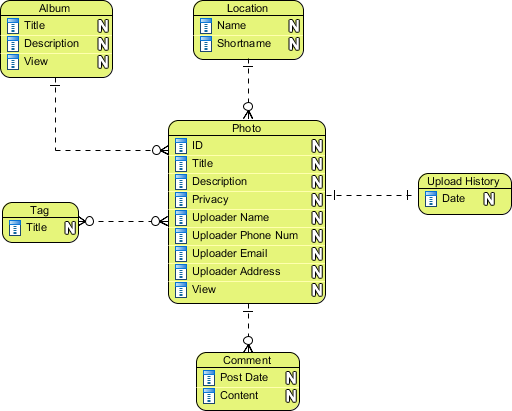
Conceptual Model

Conceptual ERD models information gathered from business requirements. Entities and relationships modeled in such ERD are defined around the business's need. The need of satisfying the database design is not considered yet. Conceptual ERD is the simplest model among all.

Conceptual ERD example

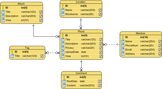
Logical Model

Logical ERD also models information gathered from business requirements. It is more complex than conceptual model in that column types are set. Note that the setting of column types is optional and if you do that, you should be doing that to aid business analysis. It has nothing to do with database creation yet.

Logical ERD example

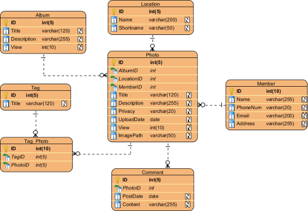
Physical Model

Physical ERD represents the actual design blueprint of a relational database. It represents how data should be structured and related in a specific DBMS so it is important to consider the convention and restriction of the DBMS you use when you are designing a physical ERD. This means that an accurate use of data type is needed for entity columns and the use of reserved words has to be avoided in naming entities and columns. Besides, database designers may also add primary keys, foreign keys and constraints to the design.

Physical ERD example

Attributes and Its types

Attribute : It is the name of the column. An attribute gives the characteristics of the entity. For example, A customer of bank may be described by : name, address, customer ID number. It is also called as data element, data field, a field, a data item, or an elementary item.

Type of Attributes in DBMS –

Single valued Attributes : An attribute, that has a single value for a particular entity is known as single valued attributes. For example, age of a employee entity.

Multi valued Attributes : An attributes that may have multiple values for the same entity is known as multi valued attributes. For example colors of a car entity.

Compound Attribute/Composite Attribute : Attribute can be subdivided into two or more other Attribute. For Example, Name can be divided into First name, Middle name and Last name.

Simple Attributes/Atomic Attributes : The attributes which cannot be divided into smaller subparts are called simple or atomic attributes. For example, age of employee entity

Stored Attribute : An attribute, which cannot be derived from other attribute, is known as stored attribute. For example, BirthDate of employee.

Derived Attribute : Attributes derived from other stored attribute. For example age from Date of Birth and Today’s date.

• An attribute can be derived from a single attribute. Example age from DOB and current date.
• An attribute can be derived from multiple attribute.
• An entity can be derived from a separate table. Example,
  

  RNO Name DeptNO 1 A 1 2 B 1 3 C 2 4 D 3 5 E 1

  ⇒

  DNO Dname 1 CSE 2 IT 3 ECE

Complex Attributes : If an attribute fr an entity, is built using composite and multivalued attributes, then these attributes are called complex attributes. For example, a person can have more than one residence and each residence can have multiple phones, an addressphone for a person entity can be specified as –

{Addressphone (phone {(Area Code, Phone Number)}, Address(Sector Address (Sector Number,House Number), City, State, Pin))}

Here {} are used to enclose multivalued attributes and () are used to enclose composite attributes with comma separating individual attributes./

Key Attribute : represents primary key. (main characteristics of an entity). It is an attribute, that has distinct value for each entity/element in an entity set. For example, Roll number in a Student Entity Type.

Non Key Attributes : These are attributes other than candidate key attributes in a table. For example Firstname is a non key attribute as it does not represent the main characteristics of the entity.

Required Attribute : A required attribute is an attribute that must have a data value.These attributes are required because they describe what is important in the entity. For example, In a STUDENT entity, firstname and lastname is a required attribute.

Optional Attribute/Null Value Attribute – An optional attribute may not have a value in it and can be left blank. For example, In a STUDENT entity, Middlename or email address is an optional attribute. as some students may not have middlename or email address.

Notations Of Attributes in ER Diagram 

	Attribute
	Key Attribute
	Multivalued Attribute
	Compound/Composite Attribute
	Derived Attribute

Database Keys

Introduction

For the purposes of clarity we will refer to keys in terms of RDBMS tables but the same definition, principle and naming applies equally to Entity Modelling and Normalisation.

Keys are, as their name suggests, a key part of a relational database and a vital part of the structure of a table. They ensure each record within a table can be uniquely identified by one or a combination of fields within the table. They help enforce integrity and help identify the relationship between tables. There are three main types of keys, candidate keys, primary keys and foreign keys. There is also an alternative key or secondary key that can be used, as the name suggests, as a secondary or alternative key to the primary key

Super Key

A Super key is any combination of fields within a table that uniquely identifies each record within that table.

Candidate Key

A candidate is a subset of a super key. A candidate key is a single field or the least combination of fields that uniquely identifies each record in the table. The least combination of fields distinguishes a candidate key from a super key. Every table must have at least one candidate key but at the same time can have several.

As an example we might have a student_id that uniquely identifies the students in a student table. This would be a candidate key. But in the same table we might have the student’s first name and last name that also, when combined, uniquely identify the student in a student table. These would both be candidate keys.

In order to be eligible for a candidate key it must pass certain criteria.

• It must contain unique values
• It must not contain null values
• It contains the minimum number of fields to ensure uniqueness
• It must uniquely identify each record in the table

Once your candidate keys have been identified you can now select one to be your primary key

Primary Key

A primary key is a candidate key that is most appropriate to be the main reference key for the table. As its name suggests, it is the primary key of reference for the table and is used throughout the database to help establish relationships with other tables. As with any candidate key the primary key must contain unique values, must never be null and uniquely identify each record in the table.

As an example, a student id might be a primary key in a student table, a department code in a table of all departments in an organisation. This module has the code DH3D 35 that is no doubt used in a database somewhere to identify RDBMS as a unit in a table of modules. In the table below we have selected the candidate key student_id to be our most appropriate primary key

Primary keys are mandatory for every table each record must have a value for its primary key. When choosing a primary key from the pool of candidate keys always choose a single simple key over a composite key.

Foreign Key

A foreign key is generally a primary key from one table that appears as a field in another where the first table has a relationship to the second. In other words, if we had a table A with a primary key X that linked to a table B where X was a field in B, then X would be a foreign key in B.

An example might be a student table that contains the course_id the student is attending. Another table lists the courses on offer with course_id being the primary key. The 2 tables are linked through course_id and as such course_id would be a foreign key in the student table.

Secondary Key or Alternative Key

A table may have one or more choices for the primary key. Collectively these are known as candidate keys as discuss earlier. One is selected as the primary key. Those not selected are known as secondary keys or alternative keys.

For example in the table showing candidate keys above we identified two candidate keys, studentId and firstName + lastName. The studentId would be the most appropriate for a primary key leaving the other candidate key as secondary or alternative key. It should be noted for the other key to be candidate keys, we are assuming you will never have a person with the same first and last name combination. As this is unlikely we might consider fistName+lastName to be a suspect candidate key as it would be restrictive of the data you might enter. It would seem a shame to not allow John Smith onto a course just because there was already another John Smith.

Simple Key

Any of the keys described before (ie primary, secondary or foreign) may comprise one or more fields, for example if firstName and lastName was our key this would be a key of two fields where as studentId is only one. A simple key consists of a single field to uniquely identify a record. In addition the field in itself cannot be broken down into other fields, for example, studentId, which uniquely identifies a particular student, is a single field and therefore is a simple key. No two students would have the same student number.

Compound Key

A compound key consists of more than one field to uniquely identify a record. A compound key is distinguished from a composite key because each field, which makes up the primary key, is also a simple key in its own right. An example might be a table that represents the modules a student is attending. This table has a studentId and a moduleCode as its primary key. Each of the fields that make up the primary key are simple keys because each represents a unique reference when identifying a student in one instance and a module in the other.

Composite Key

A composite key consists of more than one field to uniquely identify a record. This differs from a compound key in that one or more of the attributes, which make up the key, are not simple keys in their own right. Taking the example from compound key, imagine we identified a student by their firstName + lastName. In our table representing students on modules our primary key would now be firstName + lastName + moduleCode. Because firstName + lastName represent a unique reference to a student, they are not each simple keys, they have to be combined in order to uniquely identify the student. Therefore the key for this table is a composite key.