Conceptual, Physical and Logical Data Models

The three level of data modeling:-

conceptual data model

A conceptual data model identifies the highest-level relationships between the different entities. Features of conceptual data model include:

·         Includes the important entities and the relationships among them.

·         No attribute is specified.

·         No primary key is specified.

logical data model

A logical data model describes the data in as much detail as possible, without regard to how they will be physical implemented in the database. Features of a logical data model include:

·         Includes all entities and relationships among them.

·         All attributes for each entity are specified.

·         The primary key for each entity is specified.

·         Foreign keys (keys identifying the relationship between different entities) are specified.

·         Normalization occurs at this level.

The steps for designing the logical data model are as follows:

1.     Specify primary keys for all entities.

2.     Find the relationships between different entities.

3.     Find all attributes for each entity.

4.     Resolve many-to-many relationships.

5.     Normalization.

physical data model

Physical data model represents how the model will be built in the database. A physical database model shows all table structures, including column name, column data type, column constraints, primary key, foreign key, and relationships between tables. Features of a physical data model include:

• Specification all tables and columns.
• Foreign keys are used to identify relationships between tables.
• Denormalization may occur based on user requirements.
• Physical considerations may cause the physical data model to be quite different from the logical data model.
• Physical data model will be different for different RDBMS. For example, data type for a column may be different between Oracle, DB2 etc.

The steps for physical data model design are as follows:

1. Convert entities into tables.
2. Convert relationships into foreign keys.
3. Convert attributes into columns.
4. Modify the physical data model based on physical constraints / requirements.

Here we compare these three types of data models. The table below compares the different features:

Feature	Conceptual	Logical	Physical
Entity Names	✓	✓
Entity Relationships	✓	✓
Attributes		✓
Primary Keys		✓	✓
Foreign Keys		✓	✓
Table Names			✓
Column Names			✓
Column Data Types			✓

Conceptual Model Design 

Logical Model Design

Physical Model Design

We can see that the complexity increases from conceptual to logical to physical. This is why we always first start with the conceptual data model (so we understand at high level what are the different entities in our data and how they relate to one another), then move on to the logical data model (so we understand the details of our data without worrying about how they will actually implemented), and finally the physical data model (so we know exactly how to implement our data model in the database of choice). In a data warehousing project, sometimes the conceptual data model and the logical data model are considered as a single deliverable.

Conclusion:

Conceptual, logical and physical model or ERD are three different ways of modeling data in a domain. While they all contain entities and relationships, they differ in the purposes they are created for and audiences they are meant to target. A general understanding to the three models is that, business analyst uses conceptual and logical model for modeling the data required and produced by system from a business angle, while database designer refines the early design to produce the physical model for presenting physical database structure ready for database construction.

With Visual Paradigm, you can draw the three types of model, plus to progress through models through the use of Model Transitor.

Conceptual Model

Conceptual ERD models information gathered from business requirements. Entities and relationships modeled in such ERD are defined around the business's need. The need of satisfying the database design is not considered yet. Conceptual ERD is the simplest model among all.

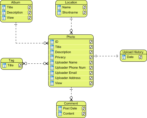
Conceptual ERD example

Logical Model

Logical ERD also models information gathered from business requirements. It is more complex than conceptual model in that column types are set. Note that the setting of column types is optional and if you do that, you should be doing that to aid business analysis. It has nothing to do with database creation yet.

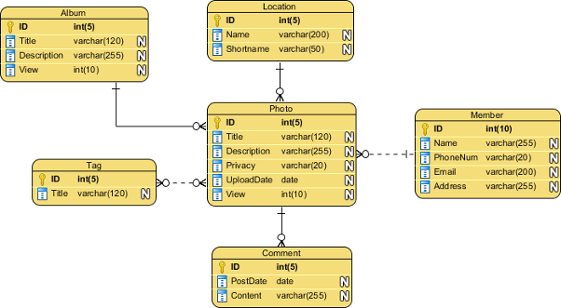
Logical ERD example

Physical Model

Physical ERD represents the actual design blueprint of a relational database. It represents how data should be structured and related in a specific DBMS so it is important to consider the convention and restriction of the DBMS you use when you are designing a physical ERD. This means that an accurate use of data type is needed for entity columns and the use of reserved words has to be avoided in naming entities and columns. Besides, database designers may also add primary keys, foreign keys and constraints to the design.

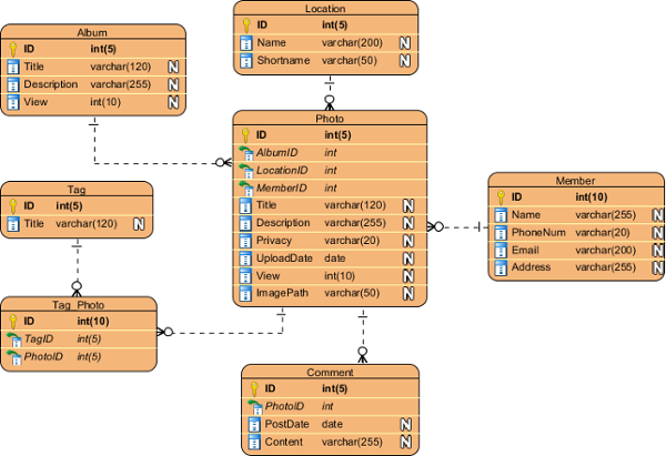
Physical ERD example

Attributes and Its types

Attribute : It is the name of the column. An attribute gives the characteristics of the entity. For example, A customer of bank may be described by : name, address, customer ID number. It is also called as data element, data field, a field, a data item, or an elementary item.

Type of Attributes in DBMS –

Single valued Attributes : An attribute, that has a single value for a particular entity is known as single valued attributes. For example, age of a employee entity.

Multi valued Attributes : An attributes that may have multiple values for the same entity is known as multi valued attributes. For example colors of a car entity.

Compound Attribute/Composite Attribute : Attribute can be subdivided into two or more other Attribute. For Example, Name can be divided into First name, Middle name and Last name.

Simple Attributes/Atomic Attributes : The attributes which cannot be divided into smaller subparts are called simple or atomic attributes. For example, age of employee entity

Stored Attribute : An attribute, which cannot be derived from other attribute, is known as stored attribute. For example, BirthDate of employee.

Derived Attribute : Attributes derived from other stored attribute. For example age from Date of Birth and Today’s date.

• An attribute can be derived from a single attribute. Example age from DOB and current date.
• An attribute can be derived from multiple attribute.
• An entity can be derived from a separate table. Example,
  

  RNO Name DeptNO 1 A 1 2 B 1 3 C 2 4 D 3 5 E 1

  ⇒

  DNO Dname 1 CSE 2 IT 3 ECE

Complex Attributes : If an attribute fr an entity, is built using composite and multivalued attributes, then these attributes are called complex attributes. For example, a person can have more than one residence and each residence can have multiple phones, an addressphone for a person entity can be specified as –

{Addressphone (phone {(Area Code, Phone Number)}, Address(Sector Address (Sector Number,House Number), City, State, Pin))}

Here {} are used to enclose multivalued attributes and () are used to enclose composite attributes with comma separating individual attributes./

Key Attribute : represents primary key. (main characteristics of an entity). It is an attribute, that has distinct value for each entity/element in an entity set. For example, Roll number in a Student Entity Type.

Non Key Attributes : These are attributes other than candidate key attributes in a table. For example Firstname is a non key attribute as it does not represent the main characteristics of the entity.

Required Attribute : A required attribute is an attribute that must have a data value.These attributes are required because they describe what is important in the entity. For example, In a STUDENT entity, firstname and lastname is a required attribute.

Optional Attribute/Null Value Attribute – An optional attribute may not have a value in it and can be left blank. For example, In a STUDENT entity, Middlename or email address is an optional attribute. as some students may not have middlename or email address.

Notations Of Attributes in ER Diagram 

	Attribute
	Key Attribute
	Multivalued Attribute
	Compound/Composite Attribute
	Derived Attribute

Database Keys

Introduction

For the purposes of clarity we will refer to keys in terms of RDBMS tables but the same definition, principle and naming applies equally to Entity Modelling and Normalisation.

Keys are, as their name suggests, a key part of a relational database and a vital part of the structure of a table. They ensure each record within a table can be uniquely identified by one or a combination of fields within the table. They help enforce integrity and help identify the relationship between tables. There are three main types of keys, candidate keys, primary keys and foreign keys. There is also an alternative key or secondary key that can be used, as the name suggests, as a secondary or alternative key to the primary key

Super Key

A Super key is any combination of fields within a table that uniquely identifies each record within that table.

Candidate Key

A candidate is a subset of a super key. A candidate key is a single field or the least combination of fields that uniquely identifies each record in the table. The least combination of fields distinguishes a candidate key from a super key. Every table must have at least one candidate key but at the same time can have several.

As an example we might have a student_id that uniquely identifies the students in a student table. This would be a candidate key. But in the same table we might have the student’s first name and last name that also, when combined, uniquely identify the student in a student table. These would both be candidate keys.

In order to be eligible for a candidate key it must pass certain criteria.

• It must contain unique values
• It must not contain null values
• It contains the minimum number of fields to ensure uniqueness
• It must uniquely identify each record in the table

Once your candidate keys have been identified you can now select one to be your primary key

Primary Key

A primary key is a candidate key that is most appropriate to be the main reference key for the table. As its name suggests, it is the primary key of reference for the table and is used throughout the database to help establish relationships with other tables. As with any candidate key the primary key must contain unique values, must never be null and uniquely identify each record in the table.

As an example, a student id might be a primary key in a student table, a department code in a table of all departments in an organisation. This module has the code DH3D 35 that is no doubt used in a database somewhere to identify RDBMS as a unit in a table of modules. In the table below we have selected the candidate key student_id to be our most appropriate primary key

Primary keys are mandatory for every table each record must have a value for its primary key. When choosing a primary key from the pool of candidate keys always choose a single simple key over a composite key.

Foreign Key

A foreign key is generally a primary key from one table that appears as a field in another where the first table has a relationship to the second. In other words, if we had a table A with a primary key X that linked to a table B where X was a field in B, then X would be a foreign key in B.

An example might be a student table that contains the course_id the student is attending. Another table lists the courses on offer with course_id being the primary key. The 2 tables are linked through course_id and as such course_id would be a foreign key in the student table.

Secondary Key or Alternative Key

A table may have one or more choices for the primary key. Collectively these are known as candidate keys as discuss earlier. One is selected as the primary key. Those not selected are known as secondary keys or alternative keys.

For example in the table showing candidate keys above we identified two candidate keys, studentId and firstName + lastName. The studentId would be the most appropriate for a primary key leaving the other candidate key as secondary or alternative key. It should be noted for the other key to be candidate keys, we are assuming you will never have a person with the same first and last name combination. As this is unlikely we might consider fistName+lastName to be a suspect candidate key as it would be restrictive of the data you might enter. It would seem a shame to not allow John Smith onto a course just because there was already another John Smith.

Simple Key

Any of the keys described before (ie primary, secondary or foreign) may comprise one or more fields, for example if firstName and lastName was our key this would be a key of two fields where as studentId is only one. A simple key consists of a single field to uniquely identify a record. In addition the field in itself cannot be broken down into other fields, for example, studentId, which uniquely identifies a particular student, is a single field and therefore is a simple key. No two students would have the same student number.

Compound Key

A compound key consists of more than one field to uniquely identify a record. A compound key is distinguished from a composite key because each field, which makes up the primary key, is also a simple key in its own right. An example might be a table that represents the modules a student is attending. This table has a studentId and a moduleCode as its primary key. Each of the fields that make up the primary key are simple keys because each represents a unique reference when identifying a student in one instance and a module in the other.

Composite Key

A composite key consists of more than one field to uniquely identify a record. This differs from a compound key in that one or more of the attributes, which make up the key, are not simple keys in their own right. Taking the example from compound key, imagine we identified a student by their firstName + lastName. In our table representing students on modules our primary key would now be firstName + lastName + moduleCode. Because firstName + lastName represent a unique reference to a student, they are not each simple keys, they have to be combined in order to uniquely identify the student. Therefore the key for this table is a composite key.

Basic Terminologies

Data: Facts, figures, statistics etc. having no particular meaning (e.g. 1, ABC, 19 etc).

Record: Collection of related data items, e.g. in the above example the three data items had no meaning. But if we organise them in the following way, then they collectively represent meaningful information.

Roll	Name	Age
1	ABC	19

Table or Relation: Collection of related records.

Roll	Name	Age
1	ABC	19
2	DEF	22
3	XYZ	28

The columns of this relation are called Fields, Attributes or Domains. The rows are called Tuples or Records.

Database: Collection of related relations. Consider the following collection of tables:

T1

Roll	Name	Age
1	ABC	19
2	DEF	22
3	XYZ	28

T2

Roll	Address
1	KOL
2	DEL
3	MUM

T3

Roll	Year
1	I
2	II
3	I

T4

Year	Hostel
I	H1
II	H2

We now have a collection of 4 tables. They can be called a “related collection” because we can clearly find out that there are some common attributes existing in a selected pair of tables. Because of these common attributes we may combine the data of two or more tables together to find out the complete details of a student. Questions like “Which hostel does the youngest student live in?” can be answered now, although Age and Hostelattributes are in different tables.

In a database, data is organized strictly in row and column format. The rows are calledTuple or Record. The data items within one row may belong to different data types. On the other hand, the columns are often called Domain or Attribute. All the data items within a single attribute are of the same data type.

What is Management System?

A management system is a set of rules and procedures which help us to create organize and manipulate the database. It also helps us to add, modify delete data items in the database. The management system can be either manual or computerized.

The management system is important because without the existence of some kind of rules and regulations it is not possible to maintain the database. We have to select the particular attributes which should be included in a particular table; the common attributes to create relationship between two tables; if a new record has to be inserted or deleted then which tables should have to be handled etc. These issues must be resolved by having some kind of rules to follow in order to maintain the integrity of the database.

Summary:

DBMS stands for Database Management System. We can break it like this DBMS = Database + Management System. Database is a collection of data and Management System is a set of programs to store and retrieve those data. Based on this we can define DBMS like this: DBMS is a collection of inter-related data and set of programs to store & access those data in an easy and effective manner.

What is the need of DBMS?
Database systems are basically developed for large amount of data. When dealing with huge amount of data, there are two things that require optimization: Storage of data and retrieval of data.

Storage: According to the principles of database systems, the data is stored in such a way that it acquires lot less space as the redundant data (duplicate data) has been removed before storage. Let’s take a layman example to understand this:
In a banking system, suppose a customer is having two accounts, one is saving account and another is salary account. Let’s say bank stores saving account data at one place (these places are called tables we will learn them later) and salary account data at another place, in that case if the customer information such as customer name, address etc. are stored at both places then this is just a wastage of storage (redundancy/ duplication of data), to organize the data in a better way the information should be stored at one place and both the accounts should be linked to that information somehow. The same thing we achieve in DBMS.

Fast Retrieval of data: Along with storing the data in an optimized and systematic manner, it is also important that we retrieve the data quickly when needed. Database systems ensure that the data is retrieved as quickly as possible.

Three Schema Approach

We know that the same thing, if viewed from different angles produces difference sights. Likewise, the database that we have created already can have different aspects to reveal if seen from different levels of abstraction. The term Abstraction is very important here. Generally it means the amount of detail you want to hide. Any entity can be seen from different perspectives and levels of complexity to make it a reveal its current amount of abstraction. Let us illustrate by a simple example.

A computer reveals the minimum of its internal details, when seen from outside. We do not know what parts it is built with. This is the highest level of abstraction, meaning very few details are visible. If we open the computer case and look inside at the hard disc, motherboard, CD drive, CPU and RAM, we are in middle level of abstraction. If we move on to open the hard disc and examine its tracks, sectors and read-write heads, we are at the lowest level of abstraction, where no details are invisible.

In the same manner, the database can also be viewed from different levels of abstraction to reveal different levels of details. From a bottom-up manner, we may find that there are three levels of abstraction or views in the database. We discuss them here.

The word schema means arrangement – how we want to arrange things that we have to store. The diagram above shows the three different schemas used in DBMS, seen from different levels of abstraction.

The lowest level, called the Internal or Physical schema, deals with the description of how raw data items (like 1, ABC, KOL, H2 etc.) are stored in the physical storage (Hard Disc, CD, Tape Drive etc.). It also describes the data type of these data items, the size of the items in the storage media, the location (physical address) of the items in the storage device and so on. This schema is useful for database application developers and database administrator.

The middle level is known as the Conceptual or Logical Schema, and deals with the structure of the entire database. Please note that at this level we are not interested with the raw data items anymore, we are interested with the structure of the database. This means we want to know the information about the attributes of each table, the common attributes in different tables that help them to be combined, what kind of data can be input into these attributes, and so on. Conceptual or Logical schema is very useful for database administrators whose responsibility is to maintain the entire database.

The highest level of abstraction is the External or View Schema. This is targeted for the end users. Now, an end user does not need to know everything about the structure of the entire database, rather than the amount of details he/she needs to work with. We may not want the end user to become confused with astounding amount of details by allowing him/her to have a look at the entire database, or we may also not allow this for the purpose of security, where sensitive information must remain hidden from unwanted persons. The database administrator may want to create custom made tables, keeping in mind the specific kind of need for each user. These tables are also known as virtual tables, because they have no separate physical existence. They are crated dynamically for the users at runtime. Say for example, in our sample database we have created earlier, we have a special officer whose responsibility is to keep in touch with the parents of any under aged student living in the hostels. That officer does not need to know every detail except the Roll, Name, Addresss and Age. The database administrator may create a virtual table with only these four attributes, only for the use of this officer.

Summary:

Data and Related Structures

Data are actually stored as bits, or numbers and strings, but it is difficult to work with data at this level.

It is necessary to view data at different levels of abstraction.

Schema:

• Description of data at some level. Each level has its own schema.

We will be concerned with three forms of schemas:

• physical,
• conceptual, and
• external.

---

Physical Data Level

The physical schema describes details of how data is stored: files, indices, etc. on the random access disk system.  It also typically describes the record layout of files and type of files (hash, b-tree, flat).

Early applications worked at this level - explicitly dealt with details. E.g., minimizing physical distances between related data and organizing the data structures within the file (blocked records, linked lists of blocks, etc.)

Problem:

• Routines are hardcoded to deal with physical representation.
• Changes to data structures are difficult to make.
• Application code becomes complex since it must deal with details.
• Rapid implementation of new features very difficult.

---

Conceptual Data Level

Also referred to as the Logical level

Hides details of the physical level.

• In the relational model, the conceptual schema presents data as a set of tables.

The DBMS maps data access between the conceptual to physical schemas automatically.

• Physical schema can be changed without changing application:
• DBMS must change mapping from conceptual to physical.
• Referred to as physical data independence.

---

External Data Level

In the relational model, the external schema also presents data as a set of relations. An external schema specifies a view of the data in terms of the conceptual level. It is tailored to the needs of a particular category of users. Portions of stored data should not be seen by some users and begins to implement a level of security and simplifies the view for these users

Examples:

• Students should not see faculty salaries.
• Faculty should not see billing or payment data.

Information that can be derived from stored data might be viewed as if it were stored.

• GPA not stored, calculated when needed.

Applications are written in terms of an external schema. The external view is computed when accessed.  It is not stored. Different external schemas can be provided to different categories of users. Translation from external level to conceptual level is done automatically by DBMS at run time. The conceptual schema can be changed without changing application:

• Mapping from external to conceptual must be changed.
• Referred to as conceptual data independence.